Puzzle Pong III - Irreversible Cube I
Table of Contents
| Github | https://gist.github.com/ambuc/84fca250c25f72b46a16dd28eb653708 |
|---|
The Puzzle⌗
Josh Mermelstein and I have decided to begin challenging each other to a series of a math/programming puzzles. Here was his most recent puzzle:
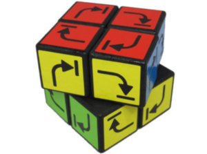
Oskar van Deventer presents an Irreversible Cube in his 2013 video which is an ordinary 2x2x2 Rubix Cube where you are only allowed to turn any face clockwise, and only once in a row.
(1) Give this cube a single twist from solved position. How many twists should it take, at minimum, to return to a solved position?
(2) For this cube, what is God’s Number?
I’ll address 1) in this post and 2) in another.
I didn’t think that the math involved in representing the cube, performing turns on it, or validating its solved-ness should be very difficult. What concerned me was difficulty in debugging these operations in the first place. Without a visualizer, it would be hard to know that my turn was working as intended. I wanted to build an engine which could take my representation of a cube and draw it, preferably in a way close to its actual 3d appearance.
Representing a Cube⌗
We represent a cube as an ordered list of points in 3d space. Implicitly, the first four are red, the second four are yellow, etc. This makes it easy to perform twists on the cube. Half the list will be on one side or another of the x, y, or z-plane, and they can be rotated about some axis while remaining put in the list.
A solved cube looks like this:
[ [ 1, 1, 2], [ 1,-1, 2], [-1, 1, 2], [-1,-1, 2]
, [ 1, 1,-2], [ 1,-1,-2], [-1, 1,-2], [-1,-1,-2]
, [ 1, 2, 1], [ 1, 2,-1], [-1, 2, 1], [-1, 2,-1]
, [ 1,-2, 1], [ 1,-2,-1], [-1,-2, 1], [-1,-2,-1]
, [ 2, 1, 1], [ 2, 1,-1], [ 2,-1, 1], [ 2,-1,-1]
, [-2, 1, 1], [-2, 1,-1], [-2,-1, 1], [-2,-1,-1]
]
Our coordinate axis is such that the very center of the cube is $(0,0,0)$, and each tile is of dimensions $2\times 2\times 0$, such that the cube is in total $4\times 4\times 4$ in dimension. This places the centers of the tiles on the faces of the subcubes at points like $(1,1,2)$; all four tiles on a the top face would have centers $(\pm 1, \pm 1, 2)$, and the four tiles on the bottom face would have centers $(\pm 1, \pm 1, -2)$.
type Coord = [Int]
type Tile  = Coord -- convenient synonym
type Cube  = [Tile]
Drawing a Cube⌗
Because the cube type carries no color information with it, the way we draw the cube is up to us. For ease of visualizing which unique tiles are which (telling apart two otherwise-identical red tiles, for example) I’ve chosen to draw each tile at a slightly different hue, generally grouped by the uniform colors a real cube might have.
I’m using the excellent Graphics.Rasterific package, which I’ve used before.
import Codec.Picture
  ( PixelRGBA8( .. ), writePng, Image)
import Graphics.Rasterific
import Graphics.Rasterific.Texture
  (uniformTexture)
import Graphics.Rasterific.Transformations
  (translate, skewX, skewY, rotate, scale)
I define some kolors which are cute little palettes of similar hues.
kolors :: [PixelRGBA8]
kolors =  [ PixelRGBA8 255 x 0 255 | x <- [000,050,100,150] ] -- reds
       ++ [ PixelRGBA8 x 0 128 255 | x <- [000,050,100,128] ] -- purples
       ++ [ PixelRGBA8 0 x 255 255 | x <- [000,050,100,128] ] -- cyans
       ++ [ PixelRGBA8 x 255 0 255 | x <- [150,170,190,210] ] -- greens
       ++ [ PixelRGBA8 255 0 x 255 | x <- [255,200,150,100] ] -- pinks
       ++ [ PixelRGBA8 x  x  x 255 | x <- [100,125,150,175] ] -- greys
And of course the solvedCube itself:
solvedCube :: Cube
solvedCube =  [ [ a, b, 2] | a <- [1,-1], b <- [1,-1] ] -- F
           ++ [ [ a, b,-2] | a <- [1,-1], b <- [1,-1] ] -- B
           ++ [ [ a, 2, b] | a <- [1,-1], b <- [1,-1] ] -- R
           ++ [ [ a,-2, b] | a <- [1,-1], b <- [1,-1] ] -- L
           ++ [ [ 2, a, b] | a <- [1,-1], b <- [1,-1] ] -- U
           ++ [ [-2, a, b] | a <- [1,-1], b <- [1,-1] ] -- D
Here’s the meat and potatoes.
Our drawing style is inspired by the following exploded isometric drawing, which I accidentally stole from a tutorial for Direct3D 11
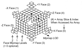
This is roughly isometric, which means we’ll need to concern ourselves with which tile to draw first, so that nearer tiles are layered over (drawn later than) further tiles.
To draw a cube (which is just an ordered list of 3d points, the centers of the 24 tiles), we zip it with the list of kolors, and then re-order the entire list by z-index, which we approximate by the sum of the three coordinates themselves. (the sortBy (comparing $ sum . fst) bit.). Then we uncurry drawTile, which takes each element of the [(coordinate, color)] list of tuples, calls drawTile crd clr, and then sweeps thru the list calling mapM_, which composes the monadic Drawing PixelRGBA8 () I/O type nicely.
:t renderDrawing    Int -> Int -> px -> Drawing px () -> Image px
:t writePng         FilePath -> Image px -> IO ()
We get a final Drawing * () which we can renderDrawing <drawing> to turn into an Image *, and finally writePng <filepath> <image>. That’s just how Rasterific handles things.
drawCube :: Cube -> Image PixelRGBA8
drawCube c = renderDrawing 600 600 (PixelRGBA8 255 255 255 255)
           $ mapM_ (uncurry drawTile)
           $ sortBy (comparing $ sum . fst)
           $ zip c kolors
OK, here’s the crazy bit. We take a coordinate crd (and a color clr to shade it, draw that as a $100x100$ pixel square in the upper-left-hand corner of the canvas, and then use a composition of several translate and scale and rotate and skewX / skewY linear matrix transformations to move the tile into the position we want it.

We compose these transformations by calling functions resize, move0, turn, skew, move1 as functions of [x,y,z], which know by how much to resize, move, turn, skew, etc. each individual tile based on its desired eventual location, angle, what have you.
It would be cool to in the future write a simple projection library which can take a 3d tuple and an assumed camera position and generate this transformation automatically. I did a bit of hand-tuning.
drawTile :: Tile -> PixelRGBA8 -> Drawing PixelRGBA8 ()
drawTile crd clr = withTransformation (center<>resize<>move0<>turn<>skew<>move1)
                 $ withTexture        (uniformTexture clr)
                 $ fill $ rectangle (V2 0 0) 100 100
  where [x ,y ,z ] = crd
        [x',y',z'] = [fromIntegral x, fromIntegral y, fromIntegral z]
        center              = translate (V2 300 300)
        resize | abs z == 2 = scale 1.0 1.0
               | otherwise  = scale 0.9 0.9
        move0  | x ==   2   = translate (V2 (-250)    50 ) --F
               | x ==  -2   = translate (V2   150  (-200)) --B
               | y ==   2   = translate (V2   150    120 ) --R
               | y ==  -2   = translate (V2 (-250) (-140)) --L
               | z ==   2   = translate (V2     0  (-230)) --U
               | z ==  -2   = translate (V2     0    120 ) --D
               | otherwise  = translate (V2     0      0 )
        turn   | abs z == 2 = rotate 0.7853
               | otherwise  = rotate 0
        skew   | abs z == 2 = skewX (-0.2) <> skewY (-0.2)
               | abs y == 2 =                 skewY (-0.6)
               | abs x == 2 =                 skewY   0.6
               | otherwise  = skewX 0
        move1  | abs z == 2 = translate (V2 ( 50*y') ( 50*x'))
               | abs y == 2 = translate (V2 (-50*x') (-50*z'))
               | abs x == 2 = translate (V2 ( 50*y') (-50*z'))
               | otherwise  = translate (V2    0        0    )
To print an image we can simply write:
main = do
   writePng "solved.png" $ drawCube solvedCube
And here’s what our solved cube looks like, finally.

Manipulation⌗
There are basically two things you can do with a $2\times 2\times 2$ cube – either turn the entire thing about an axis or twist exactly half of it about an axis.
Let’s define some new data types to make thinking about this easier.
data Side        = F | B | U | D | L | R deriving (Eq, Bounded, Show, Enum, Ord)
data Axis        = X | Y | Z
data Cardinality = Pos | Neg
type Rotation    = (Coord -> Coord)
At the most basic level, we want the ability to rotate a point clockwise or counter-clockwise exactly a quarter-turn (that is, $90^\circ$ or $\pi/2 \text{rad}$) about a line.
Pivoting⌗
There is a pretty general form for rotating a vector any turn about any line. But rather than deal with $\sin$s and $\cos$s, let’s see if we can’t limit that transformation to only quarter-turns. Using a robotics convention, we will write $\sin\theta$ as $s\theta$ and $\cos\theta$ as $c\theta$ for brevity.
$$ R_x(\theta) = \begin{bmatrix} 1&0&0 \\ 0&c\theta&-s\theta \\ 0&s\theta&c\theta\end{bmatrix} \qquad R_y(\theta) = \begin{bmatrix} c\theta&0&s\theta \\ 0&1&0 \\ -s\theta&0&c\theta \end{bmatrix} \qquad R_z(\theta) = \begin{bmatrix} c\theta&-s\theta&0 \\ s\theta&c\theta&0 \\ 0&0&1 \end{bmatrix} $$
We can apply this rotation matrix to a vector with basic matrix multiplication, like so:
$$ \begin{bmatrix}a&b&c \\ d&e&f \\ g&h&i\end{bmatrix} \begin{bmatrix}x \\ y \\ z\end{bmatrix} = \begin{bmatrix}ax+by+cz \\ dx+ey+fz \\ gx+hy+iz\end{bmatrix} $$
So what if $\theta=\pm90^\circ$? We get much simpler forms for $\pm R_x$, $\pm R_y$, and $\pm R_z$:
$$
\begin{align*}
R_x (+90^\circ) &= \begin{bmatrix}1&0&0 \\ 0&0&-1 \\ 0&1&0\end{bmatrix} &
\qquad R_x (-90^\circ) &= \begin{bmatrix}1&0&0 \\ 0&0&1 \\ 0&-1&0\end{bmatrix} \\
R_y (+90^\circ) &= \begin{bmatrix}0&0&1 \\ 0&1&0 \\ -1&0&0\end{bmatrix} &
\qquad R_y (-90^\circ) &= \begin{bmatrix}0&0&-1 \\ 0&1&0 \\ 1&0&0\end{bmatrix} \\
R_z (+90^\circ) &= \begin{bmatrix}0&-1&0 \\ 1&0&0 \\ 0&0&1\end{bmatrix} &
\qquad R_z (-90^\circ) &= \begin{bmatrix}0&1&0 \\ -1&0&0 \\ 0&0&1\end{bmatrix}
\end{align*}
$$
If we apply these simplified transformation matrices to $$\begin{bmatrix}x&y&z\end{bmatrix}^\intercal$$, we get extremely efficient, simple vector transformation anonymous functions:
mkRot :: Cardinality -> Axis -> Rotation
mkRot Pos X = \[x,y,z] -> [x,-z,y]; mkRot Neg X = \[x,y,z] -> [x,z,-y];
mkRot Pos Y = \[x,y,z] -> [z,y,-x]; mkRot Neg Y = \[x,y,z] -> [-z,y,x];
mkRot Pos Z = \[x,y,z] -> [-y,x,z]; mkRot Neg Z = \[x,y,z] -> [y,-x,z];
Writing the pivot function, which looks like newCube = pivot <cardinality> <axis> oldCube, for example, is really just a map:
pivot :: Cardinality -> Axis -> Cube -> Cube
pivot r a = map (mkRot r a)
Twisting⌗
Let’s look into the future just a little bit.
It’s the future. We’ve written our pivot/twist functions and we start exploring the space of possible cubes. Oh no! We have two cubes and we want to know if they’re the same. It’s possible that they are the same colors in the same configuration, but one is the pivoted version of another. If we just compare the points one by one, they won’t match up. And we can’t possibly generate all 24 possible pivots of $\text{cube}_A$ just to see if any of them matches $\text{cube}_B$.
What we really want is a default position for any cube. resolve takes a cube and returns that same cube, rotated according to a regular set of rules. In this case, we want to rotate the cube so that the center of the very first tile in it (the first red tile, or what have you) is located at point $(1,1,2)$.
If it’s not, but it’s located at $(?,?,2)$, we give the whole thing a clockwise Z-axis pivot and check again. It’ll get there eventually. If it’s located at $(?,?,-2)$, we flip it and try again. (Etc, etc.)
This iterative algorithm is on average quite a bit faster than checking all 24 possible pivots of a cube.
resolve :: Cube -> Cube
resolve c = resolve' $ head c
  where resolve' [ 1, 1, 2] = c
        resolve' [ _, _, 2] = resolve $ pivot Pos Z c
        resolve' [ _, _,-2] = resolve $ pivot Pos X $ pivot Pos X c
        resolve' [ _, 2, _] = resolve $ pivot Pos X c
        resolve' [ _,-2, _] = resolve $ pivot Neg X c
        resolve' [ 2, _, _] = resolve $ pivot Neg Y c
        resolve' [-2, _, _] = resolve $ pivot Pos Y c
OK, now we can write our twist function.
twist :: Side -> Cube -> Cube
twist side = resolve . map (\x -> if isOn side x then s2Rot side x else x)
  where
    isOn :: Side -> (Coord -> Bool)
    isOn F = (>0) . (!!0); isOn R = (>0) . (!!1); isOn U = (>0) . (!!2);
    isOn B = (<0) . (!!0); isOn L = (<0) . (!!1); isOn D = (<0) . (!!2);

    s2Rot :: Side -> Rotation
    s2Rot F = mkRot Pos X; s2Rot B = mkRot Neg X;
    s2Rot R = mkRot Pos Y; s2Rot L = mkRot Neg Y;
    s2Rot U = mkRot Pos Z; s2Rot D = mkRot Neg Z;
We need two helper functions, isOn and s2Rot, which only need to be scoped here. isOn takes a side and returns a function which, given a coordinate, evaluates whether or not that coordinate is on that side or not. s2Rot takes a side and returns a rotation function, so that s2Rot <side> <coord> does what you’d expect.
Solving a Cube⌗
To solve a cube we need to define what a solved cube looks like. Luckily we already know what a solved cube looks like – because tiles are indexed and we expect to always pass them around in their resolved position, we can simply write:
solved :: Cube -> Bool
solved = (== solvedCube)
That’s a great first step.
Solving the Return from a Single Offset Problem⌗
To recall the video, our current problem is to find the minimum number of moves it might take to, given a solved cube with a single twist in any direction, return to a solved position.
How do we explore the space of cubes? Well, for a 2x2 cube there’s actually only:
$$ \dfrac{ 8! \times 3^7 }{ 24 } = 7! \times 3^6 = 3,764,160$$
possible turns. Even trying all of thes positions just isn’t that bad. As we end up doing more complex things, we’ll spend more time optimizing this, but for now let’s just a) take our starter cube, b) give it all possible twists from that position, c) take all possible twists from those positions, etc. until we find a cube which is solved.
Here’s the caveat: because this cube is irreversible, we have to carry a history of the last turn. For convenience, we might as well carry a history of all turns, to make it easier to animate this solution later.
Let’s make our seed cube, which is a tuple; the first item is a twisted cube (doesn’t matter what side is twisted), and the second item is a list of performed moves so far.
seed :: [(Cube, [Side])]
seed =  [ (twist U solvedCube, [U]) ]
Now let’s make a function to explore the space of possible “children” of a given cube. We’ll inspect the most recent turn, disallow it, and try the other two.
Even though a cube has six sides, we can only turn any given side clockwise, and turning the top face clockwise is actually the same as turning the bottom face clockwise. So we can really only operate on [R,F,U], not [R,F,U,L,B,D].
kids :: (Cube, [Side]) -> [(Cube, [Side])]
kids (c, h:hs) = [ (twist dir c, dir:h:hs) | dir <- delete h [R,F,U] ]
Ok, great! Let’s use iterate to explore the space; we can concatMap to apply the kids function to a list of input cubes and get out a flat list of output cubes. iterate applies the function to its own output over and over and returns a list of outputs; concat flattens the stream, and we can filter by which cubes are solved and print just the head (the snd of which is the winning sequence itself).
main = do
   print $ snd $ head $ filter (solved.fst)
         $ concat $ iterate (concatMap kids) seed
    j@mes $ ghc -O2 l.hs && time ./l
    [1 of 1] Compiling Main             ( l.hs, l.o )
    Linking l ...
    [F,R,F,R,F,R,U,F,R,F,R,F,R,U]

    real	0m0.551s
    user	0m0.547s
    sys	0m0.003s
This is super fast, so I don’t really care yet about optimizing. But I do want to see what it looks like.
main = do
   let seq = snd $ head $ filter (solved.fst)
           $ concat $ iterate (concatMap kids) seed
   mapM_ ( \(n,c) -> writePng ("frame" ++ show n ++ ".png")
                   $ drawCube $ resolve c
         ) $ zip [10..] $ scanr twist solvedCube seq
We can use scanr to gradually scan the list of turns across the solvedCube base by applying twist zero times, one time, two times, etc. We end up with a list of altered cubes, which we can zip with a list of indices. We can use mapM_ (which is a synonym for sequence_ . map) to write each cube out to a .png using writePng <filename> drawCube <cube>. Then we can run convert -delay 10 -loop 0 frame* animation.gif (bash, not Haskell) and get:

And that’s the 13-turn sequence it takes, at minimum, to return to a solved position from a single initial offset from a solved irreversible cube.
Conclusions⌗
The next entry will deal with finding God’s Number.