Simulated Annealing for Image Tracing

I wrote a bit of Python to help “trace” an image (perform a raster-to-vector transformation) using simulated annealing.

If you already know about image tracing, image formats, and simulated annealing, feel free to skip ahead to work. Otherwise, read on.

Background⌗

Image tracing⌗

Raster images⌗

Raster images (such as digital photos) are stored in the computer as grids of pixels. Since a raster image lives in a grid, it necessarily has a fixed size (number of pixels) and resolution (number of pixels per inch). Image resolution relates to how much detail a photograph has. An image with higher resolution can be printed larger before it begins to appear pixellated or blocky.

Vector images⌗

Vector images are not grids of pixels. They are instructions to a graphics processor for visiting points, drawing lines between them, shading areas, etc. Since points and lines are stored in the vector format as floating-point numbers, vector images have dramatically higher resolution than raster images. They can be printed at arbitrary size without pixellation since they do not consist of pixels.

Rasterization⌗

Rasterization refers to the process of converting a vector image to a raster image. This might be useful for rendering a vector to any destination which requires a grid of inputs such as an LCD screen or an inkjet printer. Rasterization is an interesting field full of optimizations (antialiasing or subpixel resolution) but it is essentially straightforward: we want to find a target raster which looks most like its source vector to the human eye.

Image tracing⌗

Image tracing refers to the process of converting a raster image to a vector image. It is also essentially straightforward: we want to find the target vector which looks most like its source raster to the human eye.

But image tracing is inherently more imprecise since it involves extrapolating information from the raster which isn’t there. (i.e. image content from in-between pixels.)

Simulated annealing⌗

Simulated annealing is an optimization technique inspired by a physical phenomenon, so let’s discuss the physical phenomenon first.

Annealing⌗

Annealing is a metallurgical process for making metal more ductile (softer) by heating it up and letting it cool slowly.

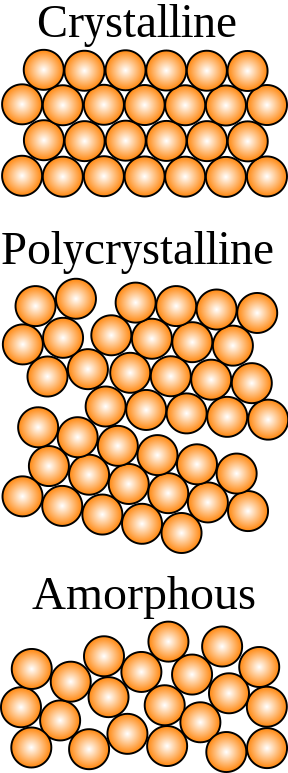
Metals usually consist of small regions of atoms called grains, where all the atoms in a grain are packed regularly. But adjacent grains are often misaligned (see the “polycrystalline” example above), leading to fracture lines called discontinuities.

When a metal is heated above some recrystallization temperature, bonds within the metal begin to break.

Cooling that metal again slowly heals fracture lines between grains, aligns adjacent grains with each other to create bigger grains, and eventually leads to a more regular (and more ductile) metal.

Simulated Annealing⌗

Simulated Annealing is an optimization technique for finding a local maximum within some search space which is too large to search completely. It is named after metallurgical annealing.

For a large and complicated search space where finding a maximum is sufficient (i.e. finding a short path between points but not necessarily the shortest possible), simulated annealing is a surprisingly effective technique.

In physical annealing, we raise and then slowly lower the temperature of a metal. In simulated annealing, temperature corresponds to the internal energy of the system, i.e. how often we spontaneously hop between candidate positions.

When simulated temperature is high, our cursor is flightier and hops between positions at random. As temperature lowers, we still seek out more optimal neighboring candidates, but our cursor “settles” and becomes increasingly unlikely to pick a new point at random.

Simulated annealing and other optimization techniques are complicated and interesting. Read much more about the techniques and history behind it here.

I won’t go into the math because this article is about a possible application of the technique rather than the technique itself.

Work⌗

With a bit of simulated annealing, we can partially automate the process of image tracing.

Here are the four kinds of image we’ll deal with:

Source  ( don't have )            Candidate  ( we generate    )
vector  ( this data  )            vector     ( this candidate )

  │                                 │
  │  ( rasterized )                 │  ( rasterized )
  │  ( by someone )                 │  ( by us      )
  │                                 │
  ▼                                 ▼

Source   ◀────(compared to)────►  Candidate
raster                            raster

The plan is as follows: We guess a series of candidate vectors and trivially rasterize them to produce a series of candidate rasters. Once we have generated a candidate raster which sufficiently resembles the source raster, we can assume its associated candiate vector also sufficiently resembles the source vector (which we cannot see).

Overview⌗

Our whole algorithm runs in a loop:

                                  Initial guess
                                  parameters
                                    │
                                    │
                      Guess new     │
   use as input  ╭──► parameters ───┤ use them
  for annealing  │                  │ to make a new
                 │                  ▼
              Fitness            Candidate
                 ▲               vector
                 │                  │
     compare to  │                  │ rasterize
  target raster  ╰─── Candidate  ◀──╯ this to produce
   to calculate       raster          a new

Eventually our measure of ‘fitness’ (more on that later) becomes sufficiently low and we decide that our candidate vector is close enough.

Caveats⌗

Here are some of the important caveats:

• we need a reasonable initial vector guess. This guess can be generated by a human or by some low-quality heuristic.

• we need a very fast way to evaluate fitness. This is the bottleneck, i.e. the majority of the time spent in the loop will be spent doing this. (Running the annealing algorithm, generating vectors, and rasterizing images are all extremely well-optimized already.)

Worked Example⌗

Take as a source vector this crude vector illustration of an ampersand, and as a source raster this even cruder rasterization.

Hopefully you can see that the raster image has lower resolution. If not, zoom in on both images until the one on the right becomes pixellated.

This is our source. Now let’s make a reasonable initial vector guess:

It doesn’t look very close. But it’s a good start.

As our simulated annealing cycle runs, we mutate each point in this initial candidate vector until the candidate raster image starts to look more and more like our source raster.

Until eventually we arrive at a final raster guess and a final vector guess.

Measuring image similarity⌗

How do we measure image similarity?

Measuring image similarity, for humans⌗

For a human, it’s really handy to look at two images with a red/blue overlay. (A red/blue overlay is a blend of two images where one input becomes the red channel of the output, and the other input becomes the blue channel of the output. Pixels which are present in both images are rendered black.)

Here are two overlays: one of the initial guess against the source image, and another of the final guess against the source image.

You can see that the initial guess (in blue) is quite poor. But our final guess is much better. You can see only a few blue or red edges peeking out.

Measuring image similarity, for computers⌗

It might be tempting to define fitness as “number of black pixels in an overlay”. But it turns out that this definition has some serious shortcomings.

Under this scheme, if two shapes don’t overlap at all, it doesn’t matter how far apart they are. The pixel overlap of two squares with an inch between them is zero, but the pixel overlap of two squares with three inches betweeen them is also zero.

Put another way: if we measure fitness in this way, then we’re not rewarding incremental improvement.

Blur⌗

The way around this is to blur both images before comparing them. Now we have a smooth transition between different colors in the image, so pixel overlap increases smoothly as our candidate converges.

There is obviously a sweet spot here. If you blur an image too much, then it becomes a mess and the annealing algorithms have no incentive to position the shapes precisely. If you blur them too little then you don’t get the benefit. This almost certainly needs to be tuned to the specific use case.

Conclusion⌗

This is a powerful technique for a very specific set of circumstances and inputs. But I don’t think this is a useful general-purpose technique for image tracing, since most people who want to trace images want the entire task automated. And the application domain needs a very fast evaluation loop, so this is probably unsuitable for scripting heavyweight professional vector editors. But for certain circumstances, it seems like a fast way to fine-tune the contents of a vector.

Code⌗

Here is some (lightly commented) code I used to perform the simulated annealing discussed in this article, as well as generate the illustrations above.

#!/usr/bin/python3
from PIL import Image
from scipy import optimize
from skimage import metrics
import cairo
import cv2
import numpy as np
import random
import scipy
import skimage
import tempfile


# Data class to hold lists of points, transform them, and print them to different kinds of images.
class DrawingData():
    def __init__(self, list_of_points):
        self._list_of_points = list_of_points
        self._degrees_of_freedom = sum(len(p) for p in self._list_of_points)
        # The width and height (in pixels) of the image.
        self._dimension = 90

    def transform(self, l):
        # Apply a mutator lambda |l| to each point.
        self._list_of_points = [l(p) for p in self._list_of_points]

    def degreesOfFreedom(self):
        # Return the number of degrees of freedom in the system.
        return self._degrees_of_freedom

    def applyDeltas(self, list_of_deltas) -> "DrawingData":
        # Apply a list of floating-point deltas to each x and y coordinate in
        # order. This application order must be consistent so that annealing
        # converges.
        return DrawingData([
            (x + list_of_deltas.pop(), y + list_of_deltas.pop())
            for (x, y) in self._list_of_points
        ])

    def mutate(self, n=5) -> "DrawingData":
        # Take each point and randomly displace it by up to |n| pixels.
        deltas = [random.uniform(-n, n)
                  for _ in range(2*self.degreesOfFreedom())]
        return self.applyDeltas(deltas)

    def writeToPng(self, list_of_filepaths):
        with cairo.ImageSurface(cairo.Format.RGB24, self._dimension, self._dimension) as surface:
            ct = cairo.Context(surface)
            ct.rectangle(0, 0, self._dimension, self._dimension)
            ct.set_source_rgb(1, 1, 1)
            ct.fill()

            ct.set_line_width(10)
            ct.set_source_rgb(0, 0, 0)
            ct.move_to(*self._list_of_points[0])
            for x, y in self._list_of_points[1:]:
                ct.line_to(x, y)
            ct.stroke()
            for filepath in list_of_filepaths:
                surface.write_to_png(filepath)

    def writeToSvg(self, list_of_filepaths):
        for filepath in list_of_filepaths:
            with cairo.SVGSurface(filepath, 90, 90) as surface:
                surface.set_document_unit(cairo.SVGUnit.PX)
                ct = cairo.Context(surface)

                ct.set_source_rgb(1, 1, 1)
                ct.paint()

                ct.set_line_width(10)
                ct.set_source_rgb(0, 0, 0)
                ct.move_to(*self._list_of_points[0])
                for x, y in self._list_of_points[1:]:
                    ct.line_to(x, y)
                ct.stroke()


def blur_image(image, s=(33, 33), f=10, n=0.5):
    # Take an image, blur it, and return a blend of the original and blurred images.
    # I think that this is slightly superior to the completely blurred image,
    # since it preserves a sharp cliff at the boundary of the unblurred shapes.
    return cv2.addWeighted(image, n, cv2.GaussianBlur(image, s, f), 1-n, 0.0)


def main():
    # Pointwise drawing of an ampersand. I sketched this on paper on an 8x8 grid, so...
    target_drawing = DrawingData([(6.3, 6.3), (5, 6), (2, 3), (1.5, 2), (2, 1), (3, .5), (4, .75), (4.5, 1.5),
                                  (4, 2.5), (1.75, 5), (2, 6), (2.5, 6.5), (3.5, 6.25), (5.5, 5), (7, 3), ])
    # ...we have to scale it up to fit on an 80x80 image.
    target_drawing.transform(lambda p: (3 + (p[0]*10), 7 + (p[1]*10)))

    target_drawing.writeToPng(['target.png'])
    target_drawing.writeToSvg(['target.svg'])

    # Keep track of the frame number, so that we can render a gif of only every
    # tenth frame. (Otherwise we store too much data in memory, and the GIF
    # takes too long to watch.)
    global frame_num
    frame_num = 0
    frame_files = []

    # This is the function scipy.optimize.minimize is minimizing, so it has to
    # return fitness as a floating-point number.
    def eval(ts, initial_guess_drawing, target_file):
        global frame_num
        frame_num += 1

        guess_file = tempfile.SpooledTemporaryFile(suffix="png")

        guess_drawing = initial_guess_drawing.applyDeltas(list(ts.tolist()))
        guess_drawing.writeToPng([guess_file, "guess.png"])
        guess_drawing.writeToSvg(["guess.svg"])

        # Open both images, blur them, and return the mean squared error.
        mse = skimage.metrics.mean_squared_error(
            blur_image(cv2.imdecode(np.frombuffer(
                guess_file._file.getbuffer(), np.uint8), -1)),
            blur_image(cv2.imdecode(np.frombuffer(
                target_file._file.getbuffer(), np.uint8), -1)))

        # The image contents of tenth frame gets moved into a big list instead
        # of garbage collected.
        if frame_num % 10 == 0:
            frame_files.append(guess_file)
        else:
            del guess_file

        return mse

    # This is a bit nontraditional -- we store target and guess images both on
    # disk (for human analysis later) and in spooled temporary files, for very
    # fast inmemory access.
    with tempfile.SpooledTemporaryFile(suffix="png") as target_file:
        target_drawing.writeToPng([target_file])

        with tempfile.SpooledTemporaryFile(suffix="png") as init_guess_file:
            init_guess_drawing = target_drawing.mutate(n=5)
            init_guess_drawing.writeToPng([init_guess_file, 'init_guess.png'])
            init_guess_drawing.writeToSvg(['init_guess.svg'])

            # It typically takes 3-8 rounds before one converges. If a round
            # doesn't converge within 1000 iterations (see `maxiter` below), we
            # make another random guess and try some more.
            round = 0
            while True:
                round += 1

                # Reset our list of frames.
                frames = []
                for frame_file in frame_files:
                    del frame_file
                frame_num = 0

                # Make another random guess. These guesses are drawn from the
                # initial random guess, so they are one step further removed
                # from our source image.
                random_start_drawing = init_guess_drawing.mutate(n=5)

                r = scipy.optimize.minimize(
                    fun=eval,
                    # Since the set of parameters we're tuning are x/y
                    # translations for the points in the image, our intial state
                    # should be a vector of zeros.
                    x0=[0]*2*random_start_drawing.degreesOfFreedom(),
                    # COBYLA was experimentally selected. There might be better methods.
                    method='COBYLA',
                    args=(random_start_drawing, target_file),
                    # Also experimentally selected.
                    tol=0.000001,
                    options={
                        # Also experimentally selected.
                        'maxiter': 1000,
                    }
                )
                # If our image is within 20 pixels MSE (also experimentally
                # selected), it is close enough.
                if r.fun < 20:
                    print("Num Trials: ", round)
                    print("Success: ", r.success)
                    print("Minimum error: ", r.fun)
                    print("# Trials", r.nfev)
                    print("Tuned parameters", r.x)
                    break
                else:
                    print("Minimum error: ", r.fun)

    # Open each of the spooled temp files as a PIL image.
    frames = [Image.open(f._file) for f in frame_files]
    # Trim the back half of the list. We spent a lot of time fine-tuning this,
    # which is important but uninteresting to watch in a GIF.
    frames = frames[:int(len(frames)/4)]
    # Render the list of images as a GIF.
    frames[0].save('out.gif', save_all=True, append_images=frames[1:], loop=0)
    # And finally clean up the images manually.
    for f in frame_files:
        del f


if __name__ == '__main__':
    main()