A Walkthrough of the Advection-Differencing Scheme
Table of Contents
$$ \def\phi{\varphi} $$
Disclaimer: This is something a little different. I’m going to step through solving a practice problem for the MJ2424 Numerical Methods final exam, partially as practice teaching (and understanding) the material, partially as practice writing scientifically, and partially for fun. I’ll be working off my own derivation, but checking my answers, so I really hope the material is accurate.
What is Computational Fluid Dynamics?⌗
CFD is the process of reducing problems in Fluid Dynamics to stepwise, iterative processes computers can solve. Specifically, it involves taking a real-life continuum and reducing it to a finite-volume calculation with a set number of cells, across each of which a very simple calculation will be performed. This allows us to turn a complex calculus problem, difficult for computational problem solving, into a linear algebra problem, which is much simpler.
The Problem⌗
As seen in Classroom Example 3 of Section 4.7 Discretising Advection of David D Apsley’s CFD Notes:
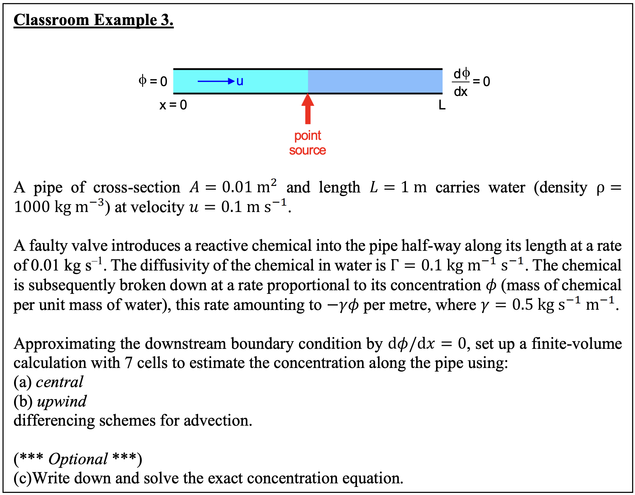
A pipe of cross-section $A = 0.01 m^2$ and length $L = 1 m$ carries water (density $\rho = 1000 kg / m^{3}$ at velocity $u = 0.1 m / s$.
A faulty valve introduces a reactive chemical into the pipe half-way along its length at a rate of $0.01 kg /s$. The diffusivity of the chemical in water is $\Gamma = 0.1 kg / m s$. The chemical is subsequently broken down at a rate proportional to its concentration $\phi$ (mass of chemical per unit mass of water), this rate amounting to $–\gamma\phi$ per metre, where $\gamma = 0.5 kg / m s$.
Assuming that the downstream boundary condition is $\d{\phi}{x}=0$, set up a finite-volume calculation with 7 cells to estimate the concentration along the pipe using:
- (a) central
- (b) upwind
differencing schemes for advection.
The Method⌗
From the normal steady-state one-dimensional advection diffusion equation
$$\pd{\rho\phi}{t} + \div(\rho\phi\v u) = div(\Gamma\grad\phi) + S_\phi $$
We make the equation steady-state and one-dimensional:
$$\d{}{x}\left(\rho u A \phi - \Gamma A \d{\phi}{x} \right)=S$$
We must now introduce the east/west convention. The current cell in question is $P$; its east and west neighbors are $E$ and $W$. Its east and west faces - that is, the boundaries it shares with those neighbors - are designated as the lowercase versions of those cardinal directions, $e$ and $w$. We can then write:
$$\d{}{x}\left( \rho u \phi \right)^e_w = \d{}{x}\left( \Gamma \d{\phi}{x} \right)^E_W$$
Integrating the transport equation, we find:
$$(\rho u A \phi)_e - (\rho u A \phi)_w = (\Gamma A)\left(\d{\phi}{x}\right)_E - (\Gamma A)\left( \d{\phi}{x} \right)$$
We define the constants: $ F = \rho A u_w^e$ and $D = \left( \frac{\Gamma A}{\Delta x} \right)_w^e$
Such that the integrated convection-diffusion equation reads:
$$F_e \phi_e - F_w \phi_w = D_e(\phi_E - \phi_P) - D_w(\phi_P - \phi_W)$$
The Central Differencing Scheme (CDS)⌗
Here we introduce a scheme for finding the values of a given property - in this problem, a chemical concentration - at a boundary between two cells, given its value at the centers of those two cells. We introduce:
$$\phi_e = \frac{\phi_E + \phi_P}{2} \qquad \phi_w = \frac{\phi_P + \phi_W}{2} \qquad \text{(This is the CDS)}$$
Expanding generally - we will expand a little more specifically in a moment - we find:
$$F_e \phi_e - F_w \phi_w = D_e (\phi_E - \phi_P) - D_w (\phi_P - \phi_w)$$
Expanding out for our CDS:
$$\frac{F_e}{2}(\phi_P + \phi_E) - \frac{F_w}{2}(\phi_W + \phi_P) = D_e(\phi_E - \phi_P) - D_w (\phi_P - \phi_W)$$
And, finally, gathering by $\phi$:
$$\left(\left(D_w + \tfrac{F_w}{2}\right)+\left(D_e - \tfrac{F_e}{2}\right)+\left(F_e - F_w\right)\right)\phi_P = \left(D_w + \tfrac{F_w}{2}\right)\phi_W + \left(D_e - \tfrac{F_e}{2}\right) \phi_E$$
Essentially, this allows us to define a set of variables, and use them repeatedly to solve this generalized cell at unique conditions, such as at boundaries or sources.
- $a_W = D_w + \tfrac{F_w}{2}$
- $a_E = D_e - \tfrac{F_e}{2}$
- $a_P = a_w + a_e + F_e - F_w$
Sources⌗
Our problem has an additional complexity - the variable in question, $\phi$, the concentration of a given chemical, has both an internal (not boundary) source, and a constant rate of dissipation. Thus we must introduce a source term. Each cell is assigned a quantity $S_u$ corresponding to the rate of material addition, and a scaling quantity $S_P$, corresponding to the dissipation of the material over space.
$$\Sigma S = S_u + S_p \phi_p$$
The problem description tells us that material is injected only once, at cell #4, at a rate of $\dot m = 0.01 kg/s$. Thus $S_u(4) = 0.01$, and $S_u = 0$ elsewhere. Additionally, the chemical dissipates at a rate $\gamma\phi$ per meter, where $\gamma = 0.5 kg / m s$. Thus, $S_P = \gamma\Delta x$, where $\Delta x$ is the step distance ($1m / 7$). $S_P$ is applicable on all cells, not just those with the chemical.
We introduce these terms on the right-hand side of the quation, as seen in the normal steady-state one-dimensional diffusion equation at the top of the page. Thus, the general form:
$$F_e \phi_e - F_w \phi_w = D_e (\phi_E - \phi_P) - D_w (\phi_P - \phi_w)$$
becomes:
$$F_e \phi_e - F_w \phi_w = D_e (\phi_E - \phi_P) - D_w (\phi_P - \phi_w) + S_u + S_P \phi_P$$
and the $S_P \phi_P$ term is often factored to the left-hand side, as above.
Solving the Problem⌗
We solve this problem on four unique cases, where we simplify $D_e = D_w$, $F_e = F_w$, and $S_p = \gamma\Delta x$ always.
The Default Cell (Cells 2, 3, 5, 6)⌗
If the cell has no sources and no boundaries, the transport equation is unchanged. We write:
$$F_e \phi_e - F_w \phi_w = D_e (\phi_E - \phi_P) - D_w (\phi_P - \phi_W) + S_u + S_p\phi_P$$
where $S_u = 0$. We expand by CDS and find:
$$(2D - S_P)\phi_P = (D+\tfrac{F}{2})\phi_W + (D-\tfrac{F}{2})\phi_E$$
And thus, $a_W = D+F/2$, $a_E = D-F/2$, $S_u = 0$, $a_p = a_E + a_W - S_P = 2D - S_P$.
The Injection Cell (Cell 4)⌗
The Injection Cell behaves in a very similar manner to the Default Cell, except that there is a source, so $S_u$ is nonzero. Thus: $a_W = D+F/2$, $a_E = D-F/2$, $S_u = 0.1$, $a_p = a_E + a_W - S_P = 2D - S_P$.
The Left Boundary (Cell 1)⌗
The boundary conditions are unique – on the left-hand face, designated $A$, we know $\phi(A) = 0$. We expand the standard form more slowly:
$$F_e \phi_e - F_w \phi_w = D_e (\phi_E - \phi_P) - D_w (\phi_P - \phi_W) + S_u + S_P \phi_P$$
Expanding by CDS:
$$F_e \tfrac{\phi_E + \phi_P}{2} - F_a \phi_A = D_e (\phi_E - \phi_P) - D_A \phi_A + S_u + S_p \phi_P$$
We note $\phi_A = 0$. This allows us to regroup as:
$$(3D + \tfrac{F}{2} - S_p)\phi_P = (0)\phi_W + (D-\tfrac{F}{2})\phi_E + S_u$$
Thus, $a_W = 0$, $a_E = D-F/2$, $S_u = 0$, $a_p = 3D + F/2 - S_P$.
The Right Boundary (Cell 7)⌗
The right boundary is the inverse of the left boundary. We know that $\pd{\phi}{x}(B) = 0$, so the $B$ terms similarly go to zero. Thus, $a_W = D+F/2$, $a_E = 0$, $S_u = 0$, $a_p = D + F/2 - S_P$
Numerically⌗
We know $D=\Gamma A / \Delta x = 0.007 kg/s$, $F = \rho A u = 1 kg/s$, and $S_P = \gamma\Delta x = -0.07 kg/s$. We can thus solve:
| n | $a_w$ | $a_e$ | $a_p$ | $S_u$ |
|---|---|---|---|---|
| 1 | $\ 0$ | $\ -0.493$ | $\ 0.592$ | $\ 0$ |
| 2,3,5,6 | $\ 0.507$ | $\ -0.493$ | $\ 0.085$ | $\ 0$ |
| 4 | $\ 0.507$ | $\ -0.493$ | $\ 0.085$ | $\ 0.01$ |
| 7 | $\ 0.507$ | $\ 0$ | $\ 0.578$ | $\ 0$ |
These constants hold for any instance of:
$$a_P \phi_P = a_W \phi_W + a_E \phi_E + S_u$$
Using all seven iterations of this equations, we can populate a linear equation with real numerical values, and solve:
$$ \begin{pmatrix} 0.592 & 0.493 & 0 & 0 & 0 & 0 & 0\\ -0.507 & 0.085 & 0.493 & 0 & 0 & 0 & 0\\ 0 & -0.507 & 0.085 & 0.493 & 0 & 0 & 0\\ 0 & 0 & 0 & -0.507 & 0.085 & 0.493 & 0\\ 0 & 0 & 0 & 0 & -0.507 & 0.085 & 0.493\\ 0 & 0 & 0 & 0 & 0 & -0.507 & 0.578 \end{pmatrix} \begin{bmatrix}\phi(1)\\phi(2)\\phi(3)\\phi(4)\\phi(5)\\phi(6)\\phi(7)\end{bmatrix} = \begin{pmatrix}0\\0\\0\\0.01\\0\\0\\0\end{pmatrix} $$
Which we can solve in a computer (or by hand, if you’re a sadist) to get real values for $\phi(n)$ for all values in $n = [1..7]$.