Solving One Tough Puzzle

This is a puzzle from 538’s Puzzler. The puzzle is as follows:

You play a game with four balls: One ball is red, one is blue, one is green and one is yellow. They are placed in a box. You draw a ball out of the box at random and note its color. Without replacing the first ball, you draw a second ball and then paint it to match the color of the first. Replace both balls, and repeat the process. The game ends when all four balls have become the same color. What is the expected number of turns to finish the game?

The Solution⌗

We can simplify this problem down from (all possible combinations of colors) to (all possible combinations of the number of balls of each color).

The initial state (red, yellow, green, blue) can be written as (1,1,1,1); the final state (with all balls of the same color) can be written as (4).

It turns out there are only five possible states: [(1,1,1,1),(2,1,1),(3,1),(2,2),(4)].

So the most important thing will be figuring out how often state i goes to state j. Once we get a complete list of those states and probabilities, it turns out we can draw a Markov chain, turn its edges into cells in a stochastic matrix, and then find the expected number of turns to finish. The expected number of turns to finish is also known as the expected hitting time. We will get into all that a bit later.

The Code⌗

Writing pDist⌗

First, we want to write a function which can take a state and figure out which other states it can go to and how likely it is to do that. Our function pDist does that. Since the states will soon be nodes in a graph, we refer to them as node inline.

import Control.Arrow          (second, (&&&))
import Data.Either            (rights)
import Data.List              (sort, group, permutations, delete)
import Data.Map.Strict as Map (Map, empty, fromList, keys, elems, insert, 
                               findWithDefault)
import Data.Matrix as Matrix  (Matrix, fromList, multStd, inverse, identity, 
                               submatrix, nrows)
import Data.Ratio             (Ratio, (%))
import Data.Set as Set        (Set, toList, difference, fromList)
import Prelude as P
import System.Environment     (getArgs)

Here’s our spec: pDist i will return a map where the keys are the nodes j it is possible to reach from i, and the values are the probability of reaching j from i.

First we turn the node ([1,1,1,1]) into an actual list of different “colors”. We call this toUniqueRepresentation. It takes a node like [1,1,1,1] and returns a list like [1,2,3,4].

Then we call a custom allPairings on that unique representation. This is a reduced form of Data.List.permutations which generates all possible pairings we actually care about. For example, [1,2,3,4] and [1,2,4,3] are different and might both be generated by permutations, but in practice we really only care about the order of the first two and the contents (but not order) of the rest of the list. This is done with delete, which searches through a list in $O(n)$ time to delete the first instance of a passed argument. This returns a list of potential boxes.

Then we perform the paint operation on each potential box. This involves taking two balls, painting them both the color of the first, and returning them to the box.

This paint function is done inside a larger decorate decorator, which paints, sorts, groups, replaces each group with its length, and sorts those numbers. This is computationally the bottleneck of the solution, but it is the bit of logic which attempts to resolve [A,B,B,C] and [A,A,B,C] to the same underlying distribution [2,1,1].

After decorateing each potential box, we probably end up with a long list of resultant states with a lot of repetition. We don’t want the whole list of resultant states; we want a histogram! We run it thru freqMap, which does something like:

freqMap [1,1,2] -> [(1, 2%3), (2, 1%3)], where the keys of the resultant map are the possible end states, and the values are the probabilities (as fractions).

pDist :: [Int] -> Map [Int] (Ratio Int)
pDist = freqMap . P.map decorate . allPairings . toUniqueRepresentation
  where toUniqueRepresentation      :: [Int] -> [Int]
        toUniqueRepresentation node = concat $ zipWith replicate node [1..]

        allPairings    :: [Int] -> [[Int]]
        allPairings ns = [ x : y : delete y (delete x ns) 
                         | x <- ns, y <- delete x ns
                         ]

        decorate       :: [Int] -> [Int]
        decorate       = sort . P.map length . group . sort . paint

        paint          :: [Int] -> [Int]
        paint (x:y:xs) = x:x:xs

        freqMap    :: [[Int]] -> Map [Int] (Ratio Int)
        freqMap xs = Map.fromList
                   $ P.map ( second (% length xs) . (head &&& length) )
                   $ group $ sort xs

Phew. Now that we have a function like pDist, let’s see how it behaves. Inside ghci:

*Main> pDist [1,1,1,1]
fromList [([1,1,2],1 % 1)]
*Main> pDist [1,1,2]
fromList [([1,1,2],1 % 2),([1,3],1 % 3),([2,2],1 % 6)]

Very nice. It looks like [1,1,1,1] always goes to [1,1,2], with a ratio of 1%1 or 100%. It also looks like there are lots of places [1,1,2] could go; it loops back in on itself half the time.

Writing makeArrows⌗

Eventually we want to get a list of all reachable states in the puzzle, and turn those states into a set of nodes. Once we have the nodes, we can create a graph with arrows from node to node, and think about our puzzle like that. This is shaping up to be a Markov chain, so we might as well embrace it and prepare for the stochastic matrix which is to come.

Our function makeArrows is another classic haskell until condition function seed, which applies function to seed over and over until some condition is met. We will use this to build a 2D Map, where the keys are states and the values are also maps from states to probabilities. Think about it like this:

Map key   = state i
    value = Map (key   = state j                   )
                (value = prob. of transition i -> j)

We don’t know any of this at the beginining, so we seed our function with the initial state [1,1,1,1] and let it build itself lazily. The initial 2D map is just Map.insert seed (pDist seed) Map.empty, which inserts: map[seed] = (pDist seed) into an empty map.

How do we know we’re done making this 2D map? There are lots of states in this space which are not reachable; we only care about states which either have arrows coming from or going to them. We’ll be done when every node which is the endpoint of an arrow is also the beginning of an arrow. Said another way, we’ll be done when every node j in the list of state js is also in the list of state is.

We’ll write some helper functions, is and js, which return the set of all states with arrows leaving and entering them, respectively. diff does a set difference, so we’re finished when that diff is null!

If we’re not finished, we want to take a step forwards in finishing this 2D map. We find the diff, take the first node, and perform Map.insert node (pDist node) on the old arrows 2D map.

makeArrows      :: [Int] -> Map [Int] (Map [Int] (Ratio Int))
makeArrows seed = until finished step $ Map.insert seed (pDist seed) Map.empty
  where finished    :: Map [Int] (Map [Int] (Ratio Int)) -> Bool
        finished    = P.null . diff

        step        :: Map [Int] (Map [Int] (Ratio Int)) -> Map [Int] (Map [Int] (Ratio Int))
        step arrows = Map.insert node (pDist node) arrows
          where node :: [Int]
                node = head $ Set.toList $ diff arrows

        diff        :: Map [Int] (Map [Int] (Ratio Int)) -> Set [Int]
        diff arrows = Set.difference (js arrows) (is arrows)

        is          :: Map [Int] (Map [Int] (Ratio Int)) -> Set [Int]
        is          = Set.fromList . Map.keys

        js          :: Map [Int] (Map [Int] (Ratio Int)) -> Set [Int]
        js          = Set.fromList . concatMap Map.keys . Map.elems

Trying it, we find:

*Main> makeArrows [1,1,1,1]
fromList [([1,1,1,1],fromList [([1,1,2],1 % 1)]),([1,1,2],fromList [([1,1,2],1 % 2),([1,3],1 % 3),([2,2],1 % 6)]),([1,3],fromList [([1,3],1 % 2),([2,2],1 % 4),([4],1 % 4)]),([2,2],fromList [([1,3],2 % 3),([2,2],1 % 3)]),([4],fromList [([4],1 % 1)])]

I’ll clean this up for you.

*Main> makeArrows [1,1,1,1]
fromList [ ([1,1,1,1],fromList [([1,1,2],1 % 1)])
            , ([1,1,2],  fromList [([1,1,2],1 % 2)
                                ,([1,3],  1 % 3)
                                ,([2,2],  1 % 6)])
            , ([1,3],    fromList [([1,3],  1 % 2)
                                ,([2,2],  1 % 4)
                                ,([4],    1 % 4)])
            , ([2,2],    fromList [([1,3],  2 % 3)
                                ,([2,2],  1 % 3)])
            , ([4],      fromList [([4],    1 % 1)])
            ]

This is great! We can look up a key for state i, look up another key for state j, and find a probability P_{i,j}. If it doesn’t exist, we know you can’t reach j from i. But we don’t need a 2D map, we need a matrix to do matrix arithmetic on.

Writing makeMatrix⌗

Data.Matrix has a utility fromList to take a list and turn it into an n by m matrix; we can simply turn makeArrows _ into a list with 0s in the appropriate places.

If we get a list of all possible nodes, we can do a list comprehension like [probability (or zero) from i to j | i <- nodes, j <- nodes]. We use nodes = Map.keys arrows to represent all the states we care about, and use a doubly-nested Map.findWithDefault to perform a lookup with two defaults.

If i isn’t in the map, we return an empty map to perform our second lookup on; if j isn’t in that second map, we return the zero ratio (0%1). This looks like [ Map.findWithDefault (0%1) j $ Map.findWithDefault Map.empty i arrows | i <- nodes, j <- nodes ].

Writing this with nodes and some dimension n defined inline, we get:

makeMatrix        :: Map [Int] (Map [Int] (Ratio Int)) -> Matrix (Ratio Int)
makeMatrix arrows = Matrix.fromList n n list
  where list   :: [Ratio Int]
        list   = [ Map.findWithDefault (0%1) j $ Map.findWithDefault Map.empty i arrows 
                 | i <- nodes, j <- nodes
                 ]
        n      :: Int
        n      = length nodes
        nodes :: [[Int]]
        nodes = Map.keys arrows

Let’s try it:

*Main> makeMatrix $ makeArrows [1,1,1,1]
( 0 % 1    1 % 1    0 % 1    0 % 1    0 % 1 )
( 0 % 1    1 % 2    1 % 3    1 % 6    0 % 1 )
( 0 % 1    0 % 1    1 % 2    1 % 4    1 % 4 )
( 0 % 1    0 % 1    2 % 3    1 % 3    0 % 1 )
( 0 % 1    0 % 1    0 % 1    0 % 1    1 % 1 )

This looks exactly right to me. Just for fun, let’s use dot/graphviz to draw this chain with its proper nodes and edges, for comparison to the stochastic matrix which represents it.

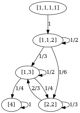
Writing expectedValue⌗

The final step will be to tease an average lifetime from this matrix. Our problem is actually asking for the expected hitting time of the Markov chain. This is the part which actually requires some math.

If we write our stochastic matrix $\textbf{P}$, we can remove the bottom row and rightmost column to remove the influence of our end state on the average lifetime. We write this reduced matrix as $\textbf{T}$, a submatrix 1 n 1 n p.

$$ \textbf{P} = \begin{bmatrix} 0 & 1 & 0 & 0 & 0\\0 & \frac{1}{2} & \frac{1}{3} & \frac{1}{6} & 0\\0 & 0 & \frac{1}{2} & \frac{1}{4} & \frac{1}{4}\\0 & 0 & \frac{2}{3} & \frac{1}{3} & 0\\0 & 0 & 0 & 0 & 1 \end{bmatrix} $$

$$ \textbf{T} = \begin{bmatrix} 0 & 1 & 0 & 0\\0 & \frac{1}{2} & \frac{1}{3} & \frac{1}{6}\\0 & 0 & \frac{1}{2} & \frac{1}{4}\\0 & 0 & \frac{2}{3} & \frac{1}{3} \end{bmatrix} $$

Here I begin quoting the Wikipedia Stochastic matrix page

• $E[k] = \tau(I + \textbf{T} + \textbf{T}^2 + …)\textbf{1}$
• $\phantom{E[k]} = \tau(I-\textbf{T})^{-1}\textbf{1}$ is the expected hitting time of the final state, where
• $\textbf{T}$ is the truncated matrix above,
• $\tau = \begin{bmatrix} 1 & 0 & 0 & 0 \end{bmatrix}$ is an array as long as the number of relevant states $n = 4$ with the initial state marked (in this case, state 1),
• $I$ is a 4x4 identity matrix, and
• $\textbf{1} = \begin{bmatrix} 1 & 1 & 1 & 1 \end{bmatrix}^{T}$ is a column vector of ones, as high as the number of relevant states $n$.

Luckily Haskell has some nice Matrix handling faculties.

expectedValue   :: Matrix (Ratio Int) -> Matrix (Ratio Int)
expectedValue p = P.foldr1 multStd [tau, inv, one]
  where tau = Matrix.fromList 1 n (1:[0,0..]) -- [1,0,0..]
        one = Matrix.fromList n 1 [1,1..]     -- [[1],[1],...]
        inv = head $ rights $ (:[]) 
            $ inverse (identity n - t)        -- (I - T)^(-1)
        t = submatrix 1 n 1 n p               -- P, but w/o last row / last col
        n = nrows p - 1                      

Tying it all together⌗

We wrap this in a main function which allows a seed to be passed in as a CLI argument, and finally call (exectedValue . makeMatrix . makeArrows) seed.

main = do
  args <- getArgs
  let seed = read (head args) :: [Int]
  print $ expectedValue $ makeMatrix $ makeArrows seed

That’s all! If we call ghc to compile it first, it takes 0.006s.

j@mes ~/dev/math-problems/four-color-balls $ ghc colorful.lhs -O2
j@mes ~/dev/math-problems/four-color-balls $ ./colorful [1,1,1,1]
( 9 % 1 )

Thus, the expected number of turns until the game is over is $9$.

You can see the complete (unannotated) haskell code on gist.